CHOIR

Installation

CHOIR is designed to be run on Unix-based operating systems such as macOS and linux.

CHOIR installation currently requires remotes and BiocManager for installation of GitHub and Bioconductor packages. Run the following commands to install the various dependencies used by CHOIR:

First, install remotes (for installing GitHub packages) if it isn’t already installed:

if (!requireNamespace("remotes", quietly = TRUE)) install.packages("remotes")

Then, install BiocManager (for installing bioconductor packages) if it isn’t already installed:

if (!requireNamespace("BiocManager", quietly = TRUE)) install.packages("BiocManager")

Then, install CHOIR:

remotes::install_github("corceslab/CHOIR", ref="main", repos = BiocManager::repositories(), upgrade = "never")

Introduction

This vignette provides a basic example of how to run CHOIR, a clustering algorithm for single-cell data. CHOIR is applicable to single-cell data of any modality, including RNA, ATAC, and proteomics. It is also applicable to multi-modal data (see Advanced Options). Detailed parameter definitions are available under the Functions tab.

CHOIR is based on the premise that if clusters contain biologically different cell types or states, a machine learning classifier that considers features present in cells from each cluster should be able to distinguish the clusters with a higher level of accuracy than machine learning classifiers trained on randomly permuted cluster labels. The use of permutation testing approaches allows CHOIR to introduce statistical significance thresholds into the clustering process.

CHOIR proceeds in two main steps. First, CHOIR generates a hierarchical clustering tree spanning the network structure of the data from an initial “partition” in which all cells are in the same cluster to a partition in which all cells are demonstrably overclustered. Then, CHOIR applies a permutation testing approach using random forest classifiers across the nodes of the hierarchical clustering tree to determine the appropriate extent of each branch of the clustering tree, such that the final clusters represent statistically distinct populations.

You’ll need the following packages installed to run this tutorial:

if (!requireNamespace("scRNAseq", quietly = TRUE)) BiocManager::install("scRNAseq")
library(scRNAseq)
library(Seurat)
library(CHOIR)

Example data

To demonstrate how to run CHOIR on a single-cell RNA-seq dataset, we’ll use a small dataset consisting of mouse dopaminergic neurons, originating from an experiment by La Manno et al. (2016), and available through the Bioconductor package scRNAseq.

data_matrix <- LaMannoBrainData('mouse-adult')@assays@data$counts
colnames(data_matrix) <- seq(1:ncol(data_matrix))

Pre-processing

CHOIR takes as input a Seurat, SingleCellExperiment, or ArchR object containing one or more feature matrices. Input data should already have undergone appropriate quality control and normalization steps (unless you are using SCTransform, see Advanced Options). Note that the exact pre-processing steps used are up to the user.

This tutorial uses a Seurat object; for details related to other object types, see Advanced Options. First, we will create a Seurat object using the read count matrix. For simplicity, here we’ll just exclude cells with fewer than 100 reads and genes present in less than 5 cells.

seurat_object <- CreateSeuratObject(data_matrix, 
                                    min.features = 100,
                                    min.cells = 5)

We will now run log normalization.

seurat_object <- NormalizeData(seurat_object)

Running CHOIR

CHOIR proceeds in two main steps:

CHOIR generates a hierarchical clustering tree.
CHOIR prunes this tree through the iterative application of a permutation testing approach.

The two steps can be run together using the function CHOIR() or separately using functions buildTree() and pruneTree().

Quick start:

The CHOIR() function will run all of the steps of the CHOIR algorithm in sequence. CHOIR is highly parallelized, so efficiency greatly improves as n_cores is increased.

The default significance level used by CHOIR is alpha = 0.05 with Bonferroni multiple comparison correction. Other correction methods may be less conservative, as CHOIR applies filters that reduce the total number of tests performed (see Advanced Options).

We recommend using the default value of alpha = 0.05 with Bonferroni multiple comparison correction. For a more conservative approach, the alpha value could be decreased to 0.01 or 0.001.

If your data has multiple batches, we highly recommend using CHOIR’s built-in batch correction, using the batch_correction_method and batch_labels parameters (see Advanced Options).

seurat_object <- CHOIR(seurat_object, 
                       n_cores = 2)

Step-by-step:

Alternately, we can run each of the two main steps of CHOIR individually.

For users who already have a set of clusters generated by a different tool, and wish to assess whether these clusters are under- or over-clustered, start at Step 2 (see Advanced Options).

Step 1: Generate hierarchical clustering tree

CHOIR generates a hierarchical clustering tree by computing dimensionality reduction and nearest neighbor adjacency matrices for the data, computing clusters across a series of sampled resolutions, then reconciling those clustering results into a consensus clustering tree using package MRtree. When using the default parameter max_clusters = "auto", CHOIR applies a series of subclustering steps to ensure that the tree is not underclustered. Specifically, the silhouette score is assessed at each new level of the emerging tree. When the silhouette score is maximized, each cluster at this level is subset, a new dimensionality reduction is generated, and the cluster is then subclustered. Each of these subtrees continues to be subdivided until the farthest pair of nearest neighboring clusters is found to be overclustered using the permutation test approach.

The user can determine which method is used for dimensionality reduction and batch correction, as well as supply specific parameters for dimensionality reduction, batch correction, detecting nearest neighbors, and modularity-based clustering, as needed. If your data has multiple batches, we highly recommend using CHOIR’s built-in batch correction, using the batch_correction_method and batch_labels parameters (see Advanced Options).

Here, we will build the hierarchical clustering tree using default parameter settings.

seurat_object <- buildTree(seurat_object,
                           n_cores = 2)
#> 
#> Input data:
#>  - Object type: Seurat (v5)
#>  - # of cells: 243
#>  - # of modalities: 1
#> 
#> Proceeding with the following parameters:
#>  - Intermediate data stored under key: CHOIR
#>  - Normalization method: none
#>  - Subtree dimensionality reductions: TRUE
#>  - Dimensionality reduction method: Default
#>  - # of variable features: Default
#>  - Batch correction method: none
#>  - Maximum clusters: auto
#>  - Minimum cluster depth: 2000
#>  - Distance approximation: TRUE
#>  - Alpha: 0.05
#>  - Multiple comparison adjustment: bonferroni
#>  - Features to train RF: var
#>  - # of excluded features: 0
#>  - # of permutations: 100
#>  - # of RF trees: 50
#>  - Use variance: TRUE
#>  - Minimum accuracy: 0.5
#>  - Minimum connections: 1
#>  - Maximum repeated errors: 20
#>  - Maximum cells sampled: Inf
#>  - Downsampling rate: 1
#>  - # of cores: 2
#>  - Random seed: 1
#> 2024-01-29 12:21:26 : (Step 1/6) Running initial dimensionality reduction..
#>                       Preparing matrix using 'RNA' assay and 'data' slot..
#>                       Running PCA with 2000 variable features..
#> 2024-01-29 12:21:27 : (Step 2/6) Generating initial nearest neighbors graph..
#> 2024-01-29 12:21:27 : (Step 3/6) Identify starting clustering resolution..
#> 
#>                       Starting resolution: 0.4
#> 2024-01-29 12:21:27 : (Step 4/6) Building parent clustering tree..
#> 
#> 
#>                       Identified 3 clusters in parent tree.
#> 2024-01-29 12:21:27 : (Step 5/6) Subclustering parent tree..
#> 2024-01-29 12:21:28 : 5% (Subtree 1/3, 112 cells), 3 total clusters.
#> 2024-01-29 12:21:31 : 44% (Subtree 1/3, 112 cells), 7 total clusters.
#> 2024-01-29 12:21:31 : 50% (Subtree 2/3, 84 cells), 7 total clusters.
#> 2024-01-29 12:21:31 : 51% (Subtree 2/3, 84 cells), 7 total clusters.
#> 2024-01-29 12:21:32 : 79% (Subtree 2/3, 84 cells), 9 total clusters.
#> 2024-01-29 12:21:32 : 81% (Subtree 2/3, 84 cells), 9 total clusters.
#> 2024-01-29 12:21:32 : 83% (Subtree 3/3, 47 cells), 9 total clusters.
#> 2024-01-29 12:21:34 : 99% (Subtree 3/3, 47 cells), 13 total clusters.
#> 
#> 2024-01-29 12:21:34 : (Step 6/6) Compiling full clustering tree..
#>                       Full tree has 6 levels and 10 clusters.

Step 2: Prune hierarchical clustering tree

After constructing the hierarchical clustering tree, CHOIR iterates through each node of the clustering tree using a bottom-up approach. At each node, CHOIR computes pairwise comparisons of all child clusters by splitting cells into training and test sets, training a balanced random forest classifier on the gene expression data of the training set, and then predicting the cluster assignments of the cells in the test set. This yields a prediction accuracy score which represents the degree to which the two clusters are distinguishable.

In parallel, CHOIR shuffles the cluster labels and repeats the same process. Both comparisons are repeated using bootstrapped samples (default = 100 iterations), resulting in a permutation test that compares the true prediction accuracy for the clusters to the prediction accuracy for a chance division of the cells into two random groups.

This permutation test yields a p-value that determines whether these clusters are slated to merge or remain separate. The significance threshold used can be adjusted using the alpha parameter. We recommend using the default value of alpha = 0.05 with Bonferroni multiple comparison correction. For a more conservative approach, the alpha value could be decreased to 0.01 or 0.001.

seurat_object <- pruneTree(seurat_object, 
                           n_cores = 2)
#> 2024-01-29 12:21:34 : (Step 1/2) Preparing object..
#> 
#> Input data:
#>  - Object type: Seurat
#>  - # of cells: 243
#>  - # of modalities: 1
#>  - # of subtrees: 4
#>  - # of levels: 6
#>  - # of starting clusters: 10
#> 
#> Proceeding with the following parameters:
#>  - Intermediate data stored under key: CHOIR
#>  - Alpha: 0.05
#>  - Multiple comparison adjustment: bonferroni
#>  - Features to train RF: var
#>  - # of excluded features: 0
#>  - # of permutations: 100
#>  - # of RF trees: 50
#>  - Use variance: TRUE
#>  - Minimum accuracy: 0.5
#>  - Minimum connections: 1
#>  - Maximum repeated errors: 20
#>  - Distance awareness: 2
#>  - Distance approximation: TRUE
#>  - Maximum cells sampled: Inf
#>  - Downsampling rate: 1
#>  - # of cores: 2
#>  - Random seed: 1
#> 2024-01-29 12:21:34 : (Step 2/2) Iterating through clustering tree..
#> 2024-01-29 12:21:35 : 11% (2/6 levels) in 0.02 min. 8 clusters remaining.
#> 2024-01-29 12:21:35 : 20% (2/6 levels) in 0.02 min. 6 clusters remaining.
#> 2024-01-29 12:21:37 : 32% (3/6 levels) in 0.05 min. 6 clusters remaining.
#> 2024-01-29 12:21:37 : 40% (3/6 levels) in 0.06 min. 6 clusters remaining.
#> 2024-01-29 12:21:37 : 50% (4/6 levels) in 0.06 min. 6 clusters remaining.
#> 2024-01-29 12:21:39 : 60% (5/6 levels) in 0.09 min. 6 clusters remaining.
#> 2024-01-29 12:21:45 : 70% (5/6 levels) in 0.18 min. 6 clusters remaining.
#> 2024-01-29 12:21:46 : 80% (6/6 levels) in 0.2 min. 5 clusters remaining.
#> 2024-01-29 12:21:49 : 91% (6/6 levels) in 0.25 min. 5 clusters remaining.
#> 2024-01-29 12:21:49 : Checking for underclustering in 1 clusters.
#> 2024-01-29 12:21:50 : Additional comparisons necessary. 5 clusters remaining.
#> 2024-01-29 12:21:50 : Completed: all clusters compared.
#> 
#>  - In 2 comparisons, clusters were split due to the minimum number of nearest neighbor connections.
#>  - In 1 comparisons, clusters were merged after correction for multiple comparisons.
#>  - Final adjusted significance threshold = 0.00227.
#> 
#> 2024-01-29 12:21:50 : Identified 5 clusters.

Plot

Labels for the final clusters identified by CHOIR can be found in the meta.data slot of the Seurat object. Other CHOIR outputs are stored under the misc slot of the Seurat object.

head(seurat_object@meta.data)
#>      orig.ident nCount_RNA nFeature_RNA CHOIR_clusters_0.05
#> 1 SeuratProject       7826         3314                   3
#> 2 SeuratProject       3294         1895                   1
#> 3 SeuratProject       6776         3002                   2
#> 4 SeuratProject       7294         3192                   1
#> 5 SeuratProject       3747         1993                   1
#> 6 SeuratProject      11258         4363                   1

After clustering has finished, we can generate a UMAP dimensionality reduction and use function plotCHOIR() to plot a visualization of the clusters.

# Run UMAP
seurat_object <- runCHOIRumap(seurat_object,
                              reduction = "P0_reduction")
#> Calculating UMAP embeddings for 1 dimensionality reductions..
#> Warning: The default method for RunUMAP has changed from calling Python UMAP via reticulate to the R-native UWOT using the cosine metric
#> To use Python UMAP via reticulate, set umap.method to 'umap-learn' and metric to 'correlation'
#> This message will be shown once per session
#> Warning: No assay specified, setting assay as RNA by default.
# Plot
plotCHOIR(seurat_object)
#> Warning: Data is of class matrix. Coercing to dgCMatrix.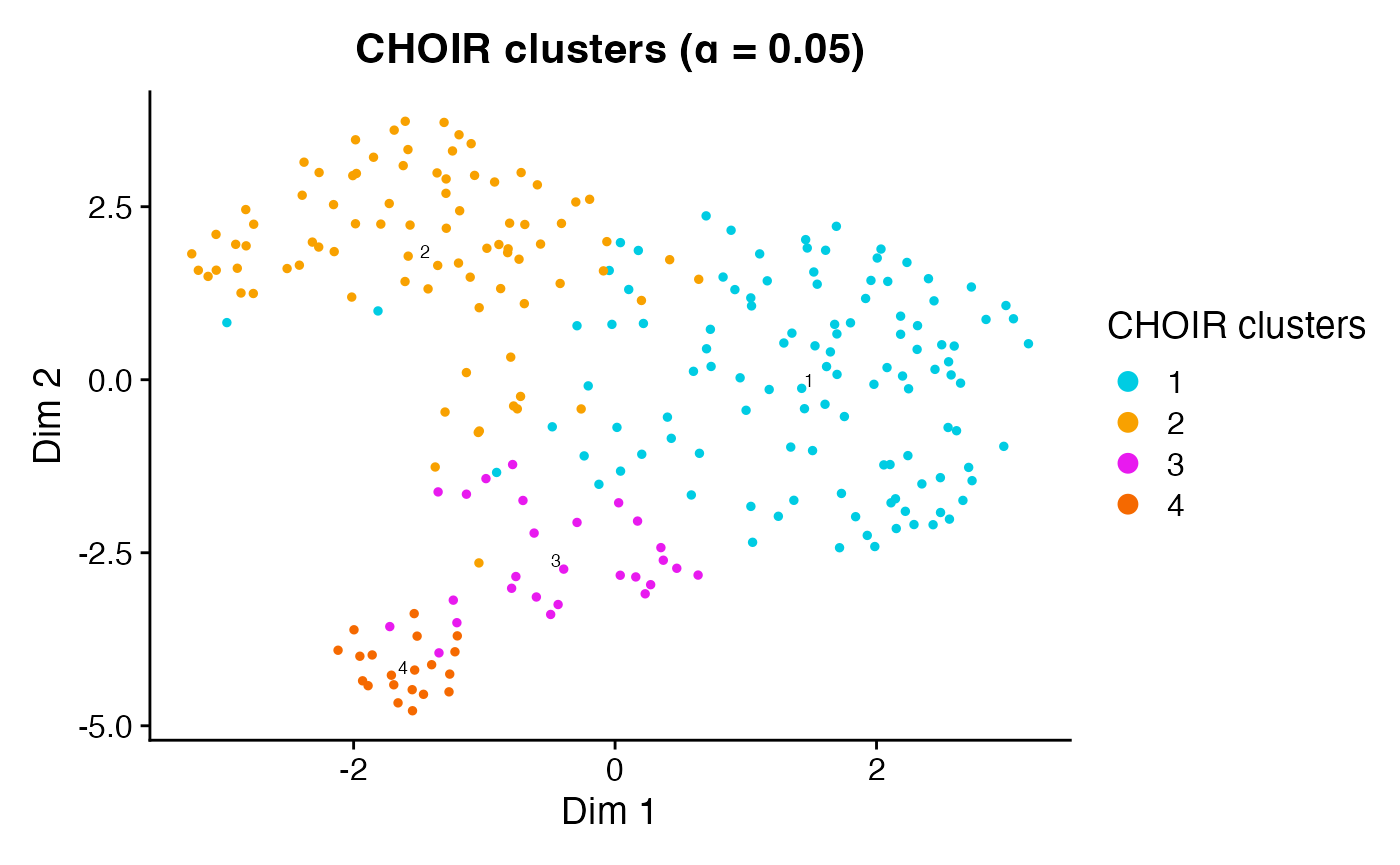

This function will also overlay the prediction accuracy scores among neighboring pairs of clusters when accuracy_scores is set to TRUE.

plotCHOIR(seurat_object,
          accuracy_scores = TRUE,
          plot_nearest = FALSE)
#> Warning: Data is of class matrix. Coercing to dgCMatrix.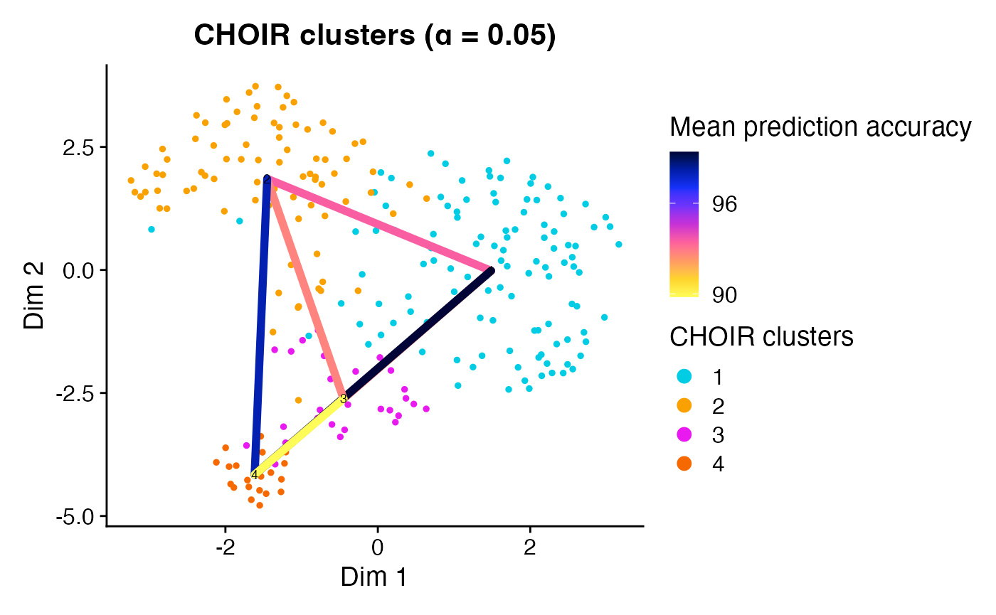

Advanced Options

Input object types

Seurat

For Seurat objects, the default assay is used if no input is provided for parameter use_assay. If no input is provided for parameter use_slot, the following default slot (Seurat v4) or layer (Seurat v5) is used:

If use_assay is either “RNA” or “sketch”, CHOIR will look for the data slot
If use_assay is either “SCT” or “integrated”, CHOIR will look for the scale.data slot

Some Seurat v5 objects have multiple layers (e.g., “data.1”, “data.2”, “data.2”..) with different subsets of cells stored under the same assay. Currently, CHOIR requires a single layer containing all cells in an assay. For these cases, please re-organize the Seurat object prior to running CHOIR.

The default dimensionality reduction method for Seurat objects is “PCA”, except in the case of ATAC-seq data, for which it is “LSI”.

If you would like to use SCTransform normalization rather than log normalization, please provide raw counts and set the parameter normalization_method = "SCTransform". Note that SCTransform has not been thoroughly tested with CHOIR.

Labels for the final clusters identified by CHOIR can be found in the meta.data slot of the Seurat object. Other CHOIR outputs are stored under the misc slot of the Seurat object.

SingleCellExperiment

For SingleCellExperiment objects, only the use_assay parameter is needed. If not provided, it is set to “logcounts”.

The default dimensionality reduction method for SingleCellExperiment objects is “PCA”, except in the case of ATAC-seq data, where it is “LSI”.

Labels for the final clusters identified by CHOIR can be found in the colData slot of the SingleCellExperiment object. Other CHOIR outputs are stored under metadata.

ArchR

For ArchR objects, if no input is provided for parameter ArchR_matrix, the “TileMatrix” is used. If no input for parameter ArchR_depthcol is provided, “nFrags” is used.

The default dimensionality reduction method for ArchR objects is “IterativeLSI”.

Labels for the final clusters identified by CHOIR can be found in the cellColData slot of the ArchR object. Other CHOIR outputs are stored under projectMetadata.

CHOIR parameters

Batch correction

For datasets with multiple batches, it is recommended to apply Harmony batch correction through CHOIR by setting the parameter batch_correction_method = "Harmony". This not only generates Harmony-corrected dimensionality reductions, but ensures that random forest classifer comparisons are batch-aware. Provide the name of the cell metadata column containing batch information to parameter batch_labels.

Use caution in applying this method if your groups of interest (e.g., disease vs. control) are batch-confounded AND you expect cell types unique to each of these groups.

Below is an example command to run CHOIR with batch correction:

seurat_object <- CHOIR(seurat_object, 
                       batch_correction_method = "Harmony",
                       batch_labels = "Batch") # Change 'Batch' to corresponding cell metadata column for your data

Significance level & multiple comparison correction

The default significance level used by CHOIR is alpha = 0.05 with Bonferroni multiple comparison correction. Other correction methods may be less conservative, as CHOIR applies filters that reduce the total number of tests performed (see below).

We recommend using the default value of alpha = 0.05 with Bonferroni multiple comparison correction. For a more conservative approach, the alpha value could be decreased to 0.01 or 0.001.

Filters

CHOIR uses various filters to reduce the number of necessary permutation test comparisons:

Parameter min_accuracy indicates the minimum accuracy for the random forest classifier predictions, below which clusters will be automatically merged. It defaults to 0.5, higher values will identify a more conservative set of clusters.
Parameter min_connections indicates the minimum number of nearest neighbors between two clusters for them to be considered ‘adjacent’. If non-zero, non-adjacent clusters will never be merged. Defaults to 1.
Parameter max_repeat_errors is used to account for situations in which random forest classifier prediction errors are concentrated among a few cells that are repeatedly misassigned (often doublets or other outliers). If non-zero, repeated errors will be evaluated and accuracy scores will be modified if the number of repeated errors is below the value of max_repeat_errors. Defaults to 20.
Parameter distance_awareness represents the distance threshold above which a cluster will not merge with another cluster. Specifically, this value is a multiplier applied to the distance between a cluster and its closest distinguishable neighbor; the product sets the threshold for subsequent comparisons. The default value sets this threshold at a 2-fold increase in distance.

Downsampling

CHOIR uses downsampling to increase efficiency for larger datasets. Using the default parameter setting of downsampling_rate = "auto", downsampling occurs at each random forest classifer comparison. The downsampling rate is determined based on the overall dataset size. To disable downsampling, set downsampling_rate = 1. For datasets that require batch correction across many batches, we recommend setting downsampling_rate = 1.

Additional downsampling can be imposed using parameter sample_max, indicating the maximum number of cells used per cluster to train/test each random forest classifier. By default, this is not used.

Providing pre-generated clusters

Users who already have a set of clusters generated by a different tool and wish to assess whether these clusters are under- or over-clustered only need to run the pruneTree() function.

To pruneTree(), provide:

object The input object under which the results will be stored.
cluster_tree A dataframe containing the cluster IDs of each cell across the levels of a hierarchical clustering tree.
input_matrix A matrix containing the feature x cell data on which to train the random forest classifiers.
nn_matrix A matrix containing the nearest neighbor adjacency of the cells.
Either reduction (a matrix of dimensionality reduction cell embeddings) if using approximate distances OR dist_matrix (a distance matrix of cell to cell distances)

Using CHOIR with ATAC-seq data

If your input data is ATAC-seq data, make sure to set input parameter atac = TRUE, in order to use the correct defaults. For example, CHOIR uses 25000 variable features by default for ATAC-seq data, in comparison to 2000 by default for other data. If your data exclusively contains ATAC-seq data (no other modalities), it is recommended to set parameter use_variance = FALSE.

CHOIR is compatible with both ArchR and Signac approaches to ATAC-seq analysis, but has been most thoroughly tested with ArchR objects.

Below is an example command to run CHOIR with ATAC-seq data:

ArchR_object <- CHOIR(ArchR_object,
                      atac = TRUE,
                      use_variance = FALSE)

If you are providing input data which contains multiple modalities from the same cell, such as RNA + ATAC multiome data, you must provide multiple values (as a vector) to parameters use_assay and use_slot (for Seurat objects), use_assay for (SingleCellExperiment objects), or ArchR_matrix and ArchR_depthcol for ArchR objects.

If you want to use different methods of normalization, dimensionality reduction, number of variable features, or batch correction for each modality, input to related parameters must also be provided as vectors or lists with one value per modality. CHOIR creates a joint dimensionality reduction for the modalities and uses all provided feature matrices as joint input to train/test random forest classifiers.

CHOIR’s approach to distance approximation is not currently compatible with multi-modal Seurat or SingleCellExperiment objects. Thus, for maximal efficiency, we recommend using ArchR objects for multi-modal analysis with CHOIR. Alternately, distance approximation can be disabled with distance_approx = FALSE, but may slow down computation.

Below is an example command to run CHOIR with joint RNA-seq and ATAC-seq data:

ArchR_object <- CHOIR(ArchR_object,
                      ArchR_matrix = c("TileMatrix", "GeneExpressionMatrix"),
                      ArchR_depthcol <- c("nFrags", "Gex_nUMI"),
                      atac = c(TRUE, FALSE))